Biwhitening
Biwhitening separates signal from noise in a data matrix whose noise variance differs from entry to entry, as it does for counts. When the noise has constant variance, its eigenvalues follow the Marchenko–Pastur law, and components of the signal stand out above the edge of that law. Unequal variances change the noise spectrum in a way that depends on the unknown pattern of variances, so that no fixed threshold separates signal from noise. The method of Landa, Zhang, and Kluger (2022) restores the law by rescaling the data:
- Estimate the noise variance of each entry.
- Scale the rows and columns of the data so that the noise has average variance one in every row and every column.
- Count the singular values of the scaled matrix that exceed the largest singular value expected of noise. Their number estimates the rank of the signal.
- Estimate the signal from those components.
Unlike a variance-stabilizing transformation, the rescaling in step 2 leaves the rank of the signal unchanged; see Comparison with variance-stabilizing transformations.
The scaling of step 2 is computed by MatrixCovers.jl, whose documentation discusses how to estimate variances for several kinds of data.
Installation
using Pkg
Pkg.add(url="https://github.com/HolyLab/Biwhitening.jl")
A first example
The example simulates counts with Poisson noise around a matrix X of expected values. X has rank 5, and its rows and columns differ widely in scale, so the noise variance differs from entry to entry.
using Biwhitening, LinearAlgebra, Random

function poisson(rng, λ)        # one Poisson variable with mean λ
    k, t = 0, randexp(rng)
    while t < λ
        k += 1
        t += randexp(rng)
    end
    return k
end

rng = Xoshiro(1)
m, n, r = 400, 1200, 5
X = (rand(rng, m, r) * rand(rng, r, n)) .* (0.2 .+ 3 .* rand(rng, m)) .* (0.2 .+ 3 .* rand(rng, n))'
Y = [poisson(rng, x) for x in X]
biwhiten assumes Poisson noise unless told otherwise:
bw = biwhiten(Y)Biwhitened{Float64} of a 400×1200 matrix
rank: 5
noise variance: 1.011
Kolmogorov–Smirnov distance to the Marchenko–Pastur law: 0.0144Five singular values of the scaled matrix exceed noise_edge, the largest singular value expected of noise:
round.(bw.S[1:8]; digits=1)', noise_edge(bw)(adjoint([1333.5, 106.8, 99.1, 98.1, 95.1, 53.9, 53.6, 53.4]), 54.64101615137755)The result holds the scales bw.a and bw.b, every singular value bw.S, and the singular vectors bw.U and bw.V of the components above the noise.
scaled(bw, Y) returns the scaled matrix itself.
Checking the variance model
The rank is meaningful only if the variances given to biwhiten describe the noise. Two numbers, both shown when a result is displayed, test this:
noise_varianceis the noise variance of the scaled matrix, estimated from its median eigenvalue. It should be close to one. A larger value means that the noise exceeds what the model predicts, and the rank is then overestimated. When the estimate changes the count, the display adds the rank for noise of the estimated variance.ks_distanceis the Kolmogorov–Smirnov distance between the eigenvalues and the Marchenko–Pastur law. Each component of the signal contributes one eigenvalue that the law does not describe, so the distance is at least the rank divided by the number of eigenvalues (here 5/400).
Neither number replaces a look at the spectrum itself. With a Makie backend loaded, spectrumplot draws it:
using CairoMakie
spectrumplot(bw)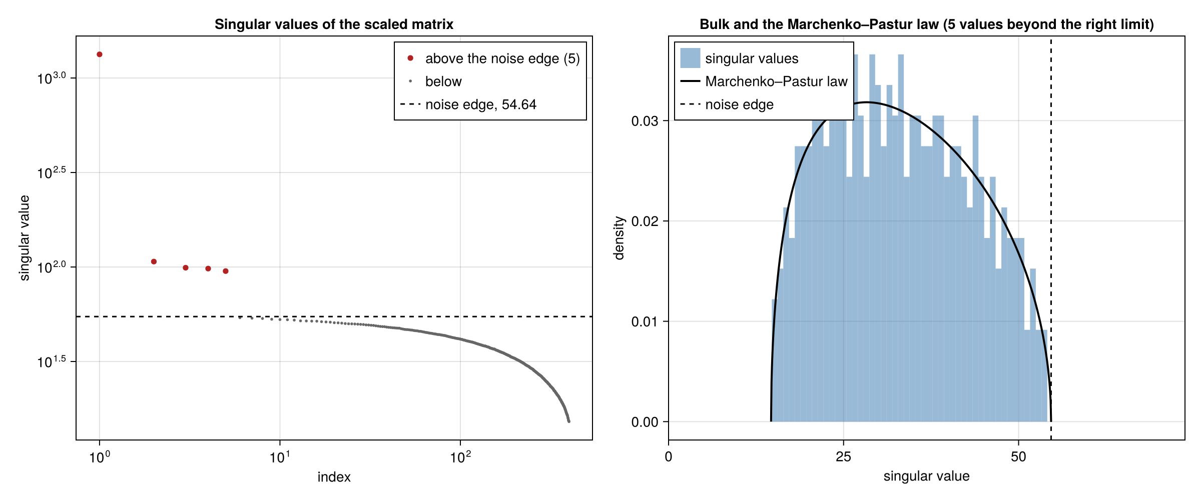
On the right, the histogram of the singular values follows the Marchenko–Pastur law up to the noise edge, as it should when the variance model describes the noise. On the left, the five components of the signal stand well clear of the edge. Real data are seldom this clear: the singular values often descend into the bulk without a gap, and the count of components then depends on exactly where the edge lies. The plot shows how many components are in that position, and whether a change of slope sets some of them apart.
d =MarchenkoPastur(bw) is the law for the eigenvalues bw.S .^ 2 ./ q, where q is the larger dimension of the matrix, and Biwhitening.pdf(d, x) is its probability density, for drawing the comparison in another way.
Choosing the variance model
Counts from sequencing are often more variable than the Poisson distribution allows. A QuadraticVariance describes noise whose variance is a quadratic function of the expected value, a + b*x + c*x^2, and fit_variance chooses b and c by comparing the spectrum with the Marchenko–Pastur law.
The counts below have a negative binomial distribution with variance x + x^2 / 4. Under the Poisson model the noise variance is far from one and the rank is wrong:
gamma4(rng) = sum(randexp(rng) for _ in 1:4) / 4     # gamma variable, shape 4, mean 1
Ynb = [poisson(rng, x * gamma4(rng)) for x in X]
biwhiten(Ynb)
Biwhitened{Float64} of a 400×1200 matrix
rank: 122 (20 if the noise has the estimated variance)
noise variance: 1.837
Kolmogorov–Smirnov distance to the Marchenko–Pastur law: 0.339The fit tries several weights β for the quadratic term and keeps the one whose spectrum is closest to the law. It starts from a coarse grid and then halves the spacing around the best candidate twice:
fit = fit_variance(Ynb)VarianceFit{Float64}: Var(y) = 1.007*x + 0.2517*x^2
β α KS distance rank
0.0 1.837 0.0666 20
0.1 1.276 0.0155 5
0.15 1.119 0.0125 5
* 0.2 1.006 0.0125 5
0.25 0.9153 0.0125 5
0.3 0.8422 0.0125 5
0.4 0.7236 0.0194 6
0.6 0.5682 0.0417 11
0.8 0.4719 0.0554 18
1.0 0.4037 0.0696 24bwnb = biwhiten(Ynb, fit.model)Biwhitened{Float64} of a 400×1200 matrix
rank: 5
noise variance: 1.0
Kolmogorov–Smirnov distance to the Marchenko–Pastur law: 0.0125The fitted coefficients are close to the true ones (b = 1, c = 0.25), the noise variance is close to one, and the rank is recovered.
Three caveats apply to the fit:
fit.scanlists every candidate. When the distance changes little over a range ofβ, the spectrum does not determineβwithin that range. The rank is then uncertain to the extent that the candidates in that range disagree about it. Above, the candidates from 0.15 to 0.3 share the smallest distance that five components allow, 5/400, and the fit takes the middle one.- The refinement assumes that the distance has a single minimum at the spacing of the coarse grid. To examine every element of a grid of your own, pass it as
gridwithrefine=0. - Because the chosen candidate was selected for its small distance, that distance is biased downward. To assess the model without this bias, fit it on some of the rows, biwhiten the remaining rows with the fitted model, and compute their
ks_distance. - With
grid=[0], the fit keeps the variance proportional to the expected value and estimates only the constant of proportionality.
For data that are not counts, pass a matrix of variance estimates, of the same size as the data, as the second argument of biwhiten.
Estimating the signal
The singular values above the noise overestimate those of the signal, and the corresponding singular vectors are tilted away from the signal's. A Shrinker replaces each singular value by an estimate that accounts for both effects (Gavish and Donoho, 2017); shrink returns the estimates.
round.([bw.S[1:5] shrink(bw, OperatorShrinker()) shrink(bw, FrobeniusShrinker())]; digits=1)5×3 Matrix{Float64}:
1333.5 1332.9 1332.3
106.8 98.8 90.9
99.1 90.4 81.8
98.1 89.2 80.5
95.1 85.9 76.9denoise rebuilds the matrix from the components with shrunk singular values and undoes the scaling. The result estimates the expected value of the data; below, its relative error is compared with that of the data themselves:
Xhat = denoise(bw)
norm(Xhat - X) / norm(X), norm(Y - X) / norm(X)
(0.05389402704815213, 0.3850437437555887)scores gives coordinates of the rows or columns on the components, for visualization or clustering:
Z = scores(bw, 1)       # one row for each row of Y, one column for each component
size(Z)
(400, 5)With the default HardThreshold these are the principal component scores of the scaled matrix. score_noise gives the noise variance of each column of the scores. It is close to one for a component well above the edge, where distances between rows are therefore in units of the noise, and it grows as a component approaches the edge, because the estimated singular vector then turns toward the noise:
round.(score_noise(bw, 1); digits=2)'1×5 adjoint(::Vector{Float64}) with eltype Float64:
1.0 1.26 1.32 1.32 1.35The sum of these values is the expected squared length of the noise in one row of Z.
The rules differ in what they estimate best:
| rule | best estimate of |
|---|---|
FrobeniusShrinker | the signal, by the sum of squared errors of its entries |
OperatorShrinker | each singular value of the signal |
NuclearShrinker | the signal, by the sum of the singular values of the error |
GramShrinker | inner products between rows, or between columns, of the signal |
HardThreshold | none; the singular values are unchanged |
Zeros, empty rows, and sparse data
biwhiten accepts sparse matrices and matrices of integers. Rows and columns without any nonzero variance estimate receive a scale of zero and are left out of the spectrum.
For some patterns of zeros no scaling exists: for example, a row whose nonzero entries lie in too few columns. biwhiten then throws an error that names the rows or columns responsible. Either remove them, or pass the keyword shrink=δ with a small positive δ. (This keyword is unrelated to the function shrink.) It mixes the variance estimates with those of a rank-one model, so that the scaling always exists. The MatrixCovers documentation describes the condition and the meaning of δ.
Comparison with variance-stabilizing transformations
A variance-stabilizing transformation equalizes noise variances in a different way: it applies a nonlinear function to each entry, such as the square root for Poisson counts or log(1 + y), so that the noise variance is approximately the same in every entry. Biwhitening equalizes only the average variance of each row and column. In exchange, it preserves linearity, on which matrix factorization depends.
Factorization methods such as principal component analysis represent the data as a sum of components, and the rank of the signal is the number of components needed. Biwhitening divides each entry by a constant, so the expected value of the scaled matrix, X ./ (a .* b'), has the same rank as the expected value X of the data (Landa, Zhang, and Kluger, 2022, eq. 2.3), and counts that add before scaling still add after it. A nonlinear transformation f preserves neither property: f.(X) generally has higher rank than X, and the expected value of f.(Y) is not f.(X). The components found in transformed data therefore need not correspond to those of the signal, and their number need not equal its rank.
Both approaches need a model of the noise variance: the square root stabilizes Poisson noise, for example, but not overdispersed noise. Variance-stabilizing transformations are also approximate, and least accurate for small expected values, which predominate in sparse counts. Biwhitening rests instead on an asymptotic theorem, which assumes that the noise is independent from entry to entry (Landa, Zhang, and Kluger, Theorem 2.2 and Proposition 4.1). Finally, because the scales weight rows and columns unequally, the singular vectors of the scaled matrix differ from those of the unscaled signal. denoise undoes the scaling, but scores are coordinates in the scaled matrix.
Cost
For an m × n matrix with m ≤ n, biwhiten forms the dense m × m Gram matrix of the scaled data and computes all of its eigenvalues. This takes memory proportional to m^2 and time proportional to m^2 * n + m^3, whether or not the data are sparse. fit_variance repeats this for every candidate, at most ten by default.
References
- M. Gavish and D. L. Donoho, "Optimal shrinkage of singular values," IEEE Transactions on Information Theory 63 (2017) 2137–2152. doi:10.1109/TIT.2017.2653801
- B. Landa, T. T. C. K. Zhang, and Y. Kluger, "Biwhitening reveals the rank of a count matrix," SIAM Journal on Mathematics of Data Science 4 (2022) 1420–1446. doi:10.1137/21M1456807